What follows is the write up for a MODIS based forest fire prediction algorithm that a colleague and myself developed in the fall of 2019. The language is a bit more formal than a usual post on this site, but ill leave it unchanged.

—————————

Wildfires are one of the largest drivers of landscape change in Canada. They have long-term and wide reaching impacts on the natural and human environment. They are also notoriously difficult to predict, especially in remote areas. Current prediction methods involve ground based estimations of weather and forest conditions to predict the likelihood of fires. However, these methods are lacking on multiple levels. Firstly their efficacy in remote areas without weather stations is lowered. And secondly, they rely on human observations followed by broad estimations. Satellite observations provides the next step in forest fire prediction. Satellites offer global daily coverage, the ability to sense the conditions in remote areas with the same precision as easily accessible areas, spatially-continuous land surface temperatures, and multiple reflectance based indices available for more accurate mapping. In this project, we attempt to use only satellite based monitoring from a single MODIS platform to predict the likelihood of impending forest fires in Central and Western Canada. While this approach has been attempted before; previous research has only been carried out on a smaller scale. Past research includes Abdollahi et. al., Bisquert et al., Chowdhury and Hassan, and Li et al. Our team has also defined a completely new methodology for determining the spatial likelihood of forest fires using MODIS 8 day composite derived indices, temperature, and land cover classification. Across the 2019 fire season in Central and Western Canada, our model succeeded in classifying 60% of the known fires into the highest burn class, and 85 % of the known fires into the highest and second highest burn classes.

Data acquisition and pre-processing

The data used in this project was Moderate resolution imaging spectroradiometer (MODIS) which is an instrument on board both the Aqua and Terra satellites.The MODIS instrument on board each of the satellite is nearly identical. The Aqua MODIS instrument is timed so that it will observe from South to North over the equator in the afternoon while the Terra MODIS instrument observes from North to South across the equator in the morning. MODIS is therefore able to cover the entire surface of the earth every 1-2 days. Furthermore, MODIS possesses 36 spectral bands, which makes it well suited to improve our understanding of the earth's dynamics on land, oceans, and parts of the atmosphere (Modis.Nasa). 

The MODIS data used in this project is level 2, also called MOD09 which is derived from level 1 data that has been atmospherically corrected so that it can provide a surface reflectance. This project used the 8 day composites with 500 meter spatial resolution and covers the period from May 8th to September 5th 2019. Band 1-7 were used to produce the indices which were used in the analysis. In addition, land surface temperature was used from the MODIS MOD11 (Modis.Userguide).

We used four reflectance-derived indices to feed into our predictive model. These indices use the relationship of MODIS (or other) satellite bands to create maps which show a useful environmental variable. These maps are able to show variables such as moisture, vegetation, soil, leaf area, snow, shadow, among others. We used four vegetation and moisture related indices, with the rationale that there should be a negative correlation between these chosen variables and the likelihood or severity of fires. 
The Normalized Difference Vegetation Index can be described as the most well-known vegetation index. The NDVI index is sensitive to green vegetation and is shown with values between -1 and 1. Negative values in this case corresponds to water bodies, clouds, etc. (Jinru & Baofeng 2017). The NDVI is used to assess regional or global vegetation and is sensitive to certain properties of the vegetation canopy such as leaf area index, vegetation condition and biomass (Zhangyan et al. 2006).
The NDVI is generated through the differences between the reflectance in NIR and the reflectance in the RED band, which is due to vegetation absorbing visible light which the RED band falls into (Zhangyan et al. 2006). Lower NDVI values often tells that vegetation is becoming unhealthy, as the plants absorb NIR light at a higher rate (EosNDVI).
NIR and RED is respectively the Near Infrared band and the Red Band which corresponds to two different ranges of surface reflectance respectively 0,7 - 1,1 nm and 0,4 - 0,7 nm (Zhangyan et al. 2006).

The Enhanced vegetation index (EVI) is another index which was used in the model. It was developed due to NDVI not including atmospheric corrections and canopy background noise. Similarly to NDVI, this index also quantifies how green the vegetation is. EVI is therefore considered a modified NDVI, which is more sensitive to high biomass areas. It is also well suited to vegetation monitoring due to its improved capability of filtering the canopy background signal and reduced atmospheric influence. The EVI index is also one of the two vegetation indices which MODIS is providing. One shortcoming of the EVI index is that it doesn’t consider the variation in radiance due topographic effects (Matsushita et al. 2007). The EVI also does not saturate as fast as NDVI does in denser vegetation as it depends more on the NIR reflectance than on the Red absorption (Glenn et al. 2008). The EVI results are interpreted the same way as NDVI, where lower values shows unhealthy vegetation and higher values means healthy vegetation.
NIR, RED and BLUE is referring to the bands and G= 2,5, C1 = 6, C2= 7,5, L= 1 are coefficients. Where L accounts for canopy background scattering and the coefficients  C1 and C2 is minimizing the residual aerosol variations (Glenn et al. 2008).

The normalized difference water index used here is the one Gao (1996) proposed. The NDWI index’s purpose is to sense the moisture in vegetation. It’s especially sensitive to variations in liquid water content of the vegetation canopies. NDWI isn’t particularly sensitive to atmospherics changes and it doesn’t completely filter away the background soil reflectance effects which NDVI does. This index is also often used for drought monitoring. Like NDVI, the values vary from -1 to 1 and the higher the value the more moisture is there in the vegetation (Gao 1996). Which was the main reason why it was included, since it would help tracking how dry the vegetation would be.

This index uses the NIR band where the wavelength is in the range of 0.841 - 0.876 nm and SWIR band where range of the wavelength is 1.628-1.652 nm (Eos.com). This translates to band 2 and band 6 in MODIS.
Where Red is the near infrared band, SWIR1 is the short wave infrared band in wavelength 1.628-1.652 nm. SWIR2 is also a short wave infrared band in the wavelength 2105-2155. These bands translate to Band 2, 6 and 7 in MODIS.

Like the NDWI, it monitors vegetation and soil moisture, but unlike the NDWI it uses the differences between two liquid water absorption channels. This means that Band 6 and 7 are being combined to act as a single band to sense soil and vegetation moisture (Wang & Qu 2007).  According to Wang & Qu 2007 the NMDI has enhanced sensitivity to drought severity and is well suited to estimate both soil and vegetation moisture due to combining information from several infrared channels.

It is important to note the difference when using this index since for vegetation low NMDI values indicate increasing drought severity. While for bare soil higher values indicate soil drought (Wang & Qu 2007).
Along with the indices and land surface temperature, the model used the Canadian land cover map to give a higher accuracy. This map, produced by Natural Resources Canada, classifies 18 separate land cover types across Canada. For the enhancement of the prediction model, some but not all of these land cover types were reclassified to act as modifiers. This reclassification was based on burning characteristics from previous studies such as Barros 2014, and Pereira 2014 which derived land cover indices for burn likelihood. Our model, however, did not attempt to reclassify all 18 land cover types. Instead, we reclassified land cover types that would have an obvious negative association to burning, such as snow, Ice, irrigated cropland, and water. The benefits of reclassification is that the final prediction map should be free of extreme outlier data for those places that will have extremely low fire risk.

The prediction maps were created through four general automated steps using python scripting. We created a custom tool that calculated all relevant indices using bands 1,2,3,6 and 7 of each multispectral image. The tool outputted NDVI, NDWI, EVI, and NMDI images. 

The second tool rescaled all calculated indices as well as the land surface temperature raster. The rescaling was achieved by taking the maximum pixel value of each raster, and dividing each pixel in each raster by the maximum of that raster. This capped the maximum value of each raster to 1. All negative values of the indices and temperature were then reclassified to 0 (as negative values correspond to water bodies (Jinru & Baofeng 2017)). This prevented one index from overpowering the others in the final model calculation. 

The indices were then inputted to the third tool, along with the indices from the preceding week to create a change raster between weeks. This helps the model see the trends in the indices, whether they are increasing or decreasing. Our rationale for this model input was that trends of drought can quickly dry vegetation in one week, therefore increasing its likelihood to burn if the trend continues in the following week.

Finally, all calculated indices, temperature, and index changes were combined together along with the reclassified land cover mask to create the final predictive map. NDVI, NDWI, and EVI were subtracted from the model, as high values in these indices represent lower fire risk. Land surface temperature and NMDI were added in the model, as the higher temperature and NMDI values correspond to higher fire risk.

In order to develop numerical accuracy for our model, it was necessary to acquire accurate burn history for the study area. The rationale for our model, as stated above, was to predict the likelihood of forest fires occurring in any given area of West-Central Canada. This type of prediction is temporally sensitive in a dynamic climate, whos variables change quickly with the weather. Thus, it was necessary to reference the predictive maps to real life forest fires which took place a short time after the prediction date. Fire data was collected between 1 and 7 days after each prediction date, giving the model a full week of fire points to use as model accuracy validation. These fire points were taken from the MODIS product MCD64A1.

The points were clipped to the study region and subsetted into weekly databases to be used to validate each 8-day MODIS composite-based prediction map. Each point dataset was paired with the former week’s prediction map. The points were overlaid on the prediction maps, and the pixel values were extracted from the raster and added as an attribute to each point. These pixel values correspond to the fire risk at that pixel, predicted by the model.

To determine the accuracy of the model, we classified each weekly image into 4 classes, representing LOW, MEDIUM, HIGH, and VERY HIGH risk for forest fires. The points were then classified based on their pixel value obtained in the model shown in figure XXX. These classifications were combined to give an overall accuracy of the model, showing what percent of all fire history points fell in which category of our prediction maps.
The maps produced for this project have each been carefully symbolized according to a planned regime. For most of the produced maps, the symbology applied consisted of stretching with standard color schemes. The stretched display method is well suited to single raster band of continuous data.

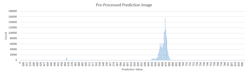
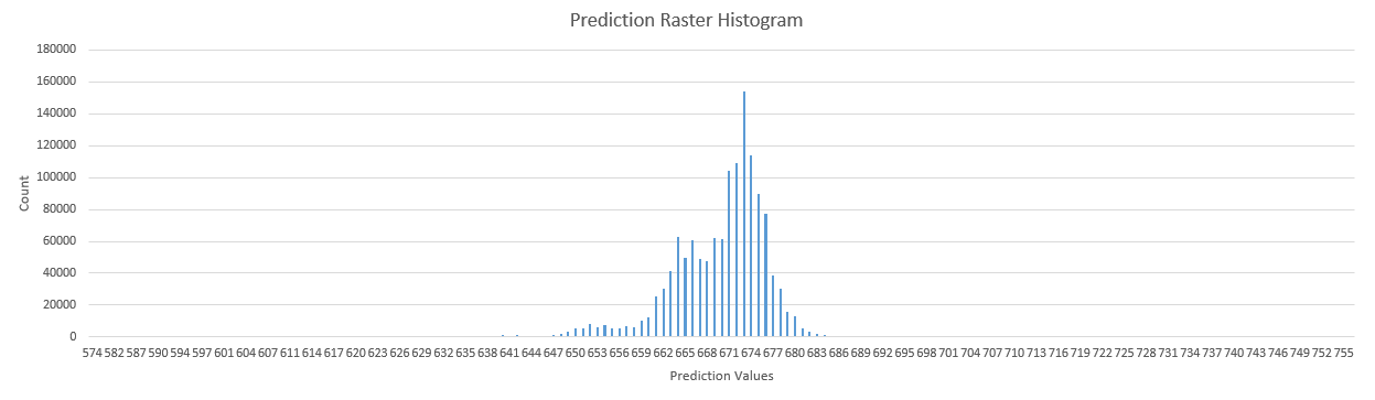
Before final symbology, all of the rasters were clipped based on 3 standard deviation above and below the mean. This removes the extreme outliers of data, allowing for more useful symbolizing. Below are the pre- and post-processed histograms of one of the prediction rasters.

The final prediction maps were all produced with the ‘histogram equalized’ symbology option, which displayed the compacted values with recognisable differences.

To validate the maps, classified symbology was used to verify whether the validation points were in either LOW, MEDIUM, HIGH or VERY HIGH categories. 

The color schemes used in this project were chosen because they matched well with the definition of how people interpret those colors compared to each other, especially in the sense of danger.

Using our method of model validation, over 85% of all known fires occured in areas that our model had classified as having ‘HIGH’ or ‘VERY HIGH’ chance of burning. Moreover, nearly 60% of all fires occurred in the ‘VERY HIGH’ class. Below are the weekly totals, and weekly percents of the forest fire points, showing the percent and count per class.

These results improved on the findings of recent papers such as Abdollahi et. al. 2018 and Chowdhury et. al. 2013. In these two papers, the researchers obtained results of 77% and 92% of their fires in their HIGH, VERY HIGH, and EXTREMELY HIGH classes respectively. Their method also used 5 classes, compared to our 4, which indicates a larger portion of their data in their ‘percent predicted’. Our method however, resulted in 85% of fires being classified in just our top 2 classes, where the former research included their top 3 classes. If we look at just the top two classes of these studies, their total drops down to 45% and 75%, respectively. Furthermore, Abdollahi et. al. used road buffers and lightning data to improve their model, under the assumption that forest fires were likely to start near roads due to human activity. We did not include these variables, and comparing our model result to Abdollahi et. al. before their inclusion of road and lightning data, our model was 10% better at fire prediction, even taking into consideration the different number of classes.

The results of the analysis showed that 85% of known fires were classified in the high, and very high risk areas of our prediction maps. This result is encouraging for this relatively simple model, especially considering it takes no ground based data into account to produce its predictions. There are however, some areas to discuss when looking into the success of the model.
Firstly, the validation points are based on real fire data over a single season. This means that the validation data isn’t evenly spread out across the time period of the study. Some of the 8 days intervals have fewer fires compared to some of the other intervals (as seen in figure 16). This could result in some of the intervals having inflated or deflated prediction scores depending on whether the few wildfires, which were registered in that period happened in areas of high risk or in areas of low risk. For example, the prediction map associated with fires which occurred on the 8th of August has a poor overall prediction success. There are very few fires in that week comparatively, and the fires that did occur were poorly predicted. This might tell us that the environmental conditions the previous week were not conducive to fires, but fires occurred the week regardless. However, when looking at the seasonal averages, we should expect the poor weekly results to be overpowered by the weeks that the model does a good job at prediction. This is exactly the phenomenon that we observe in this case, which indicates that validation error is not a strong influence in our overall result.

Another point to consider is that this project does not distinguish between man made fires and natural occurring fires. Man made fires may occur in regions and time periods that are not well correlated to our model predictions. In the case of the 8th of August, the fires which occurred could perhaps have started in areas which weren’t designated as high risk areas due to them being man made or random occurrences. This phenomenon is something this model doesn't take into account, since it is beyond the ability of the model to predict the cause of a fire, especially at a temporal resolution of 8 days.

A point to consider is the possibility that the prediction maps were completely covered in HIGH to VERY HIGH risk areas. This would result in closer to a 100 % prediction rate of fires, but would obviously not be useful in practice. This scenario was taken into consideration. We conducted tests to determine how the values from fire danger prediction maps were distributed, which can be seen in figure 12 in the symbology section. The distribution shows that the values are normally distributed, refuting the possibility of skewed predictions driving our final result.
Furthermore, it’s not out of the question that an extreme scenario could happen where there is a period with record breaking temperatures together with very low precipitation. In this case the resulting map would in fact trend strongly towards HIGH to VERY HIGH risk areas. 

Future considerations / Limitations

One of the limitations of this study was the inclusion of small fires which were likely man made, and therefore would not be accurately predicted in our model. Future research could make predictions based on large fires only, as they are more likely to be driven by larger scale (>1km) environmental factors such as the ones this study used as predictive variables. 

Another limitation of our model was the way it treated land cover classes. Some land cover classes may need different model parameters (grasslands, forests, etc.), perhaps the model could be split to only run in a single land cover type to be best matched to the known likelihoods of that particular area burning. 

Delving deeper into the vegetation indices could be necessary for future models. Firstly, tests could be run to see if some of the indices were redundant or counterproductive. Some of the indices could have been superfluous in our model and therefore including two virtually identical indices wasn't necessary. These significance test could be explored by doing an iterative process of adding indices one at a time, and seeing how much they influence the end result. This test could also determine if a different combination of indices could net better results than the one used in this project. Perhaps our original assumptions of these indices relationship to forest fire likelihood is  even wrong.
Adding other variables such as precipitation or a cloud mask may also improve the result, even though certain indices do cover how much moisture the vegetation has.
Furthermore the different parameters could be weighted differently, since some may have a higher impact than others. For instance, temperature as a parameter might have a higher impact than some of the indices, and could therefore be weighted higher in the model.

Conclusion

We achieved highly satisfactory results with our stated goal of predicting wildfires using a MODIS-only approach. 85% of all known fires between May 8th and September 5th, 2019 were classified in our two highest predictive classes. 60% of all known fires were classified in the highest predictive class. This result indicates that with the right use of variables and derived indices, a remote sensing only approach to forest fire prediction is a useful one. Although in the field of fire prediction the tides are changing in favour of a mixed ground based and satellite based approach to wildfire prediction, one of the strengths of our methodology is the standardization of prediction across large and remote areas. This is especially beneficial for areas which have little to no ground based observations of climatic or meteorological conditions. In cases where remote areas need to be considered, relying on this MODIS-only fire prediction model has a good chance of returning better results than other extant methods.